Chapter 12 Bach mouse mammary gland (10X Genomics)
12.1 Introduction
This performs an analysis of the Bach et al. (2017) 10X Genomics dataset, from which we will consider a single sample of epithelial cells from the mouse mammary gland during gestation.
12.3 Quality control
is.mito <- rowData(sce.mam)$SEQNAME == "MT"
stats <- perCellQCMetrics(sce.mam, subsets=list(Mito=which(is.mito)))
qc <- quickPerCellQC(stats, percent_subsets="subsets_Mito_percent")
sce.mam <- sce.mam[,!qc$discard]colData(unfiltered) <- cbind(colData(unfiltered), stats)
unfiltered$discard <- qc$discard
gridExtra::grid.arrange(
plotColData(unfiltered, y="sum", colour_by="discard") +
scale_y_log10() + ggtitle("Total count"),
plotColData(unfiltered, y="detected", colour_by="discard") +
scale_y_log10() + ggtitle("Detected features"),
plotColData(unfiltered, y="subsets_Mito_percent",
colour_by="discard") + ggtitle("Mito percent"),
ncol=2
)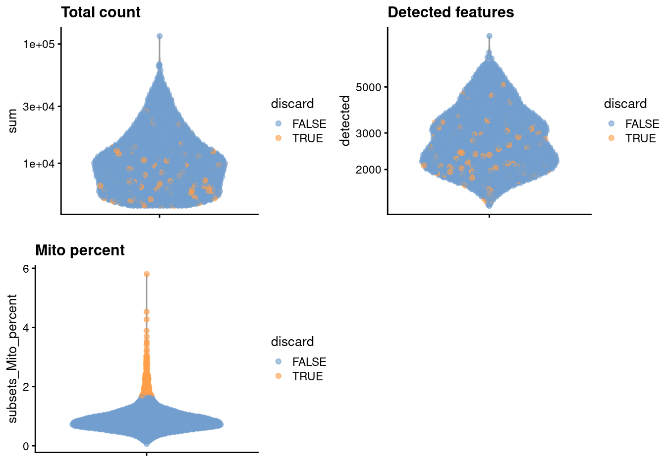
Figure 12.1: Distribution of each QC metric across cells in the Bach mammary gland dataset. Each point represents a cell and is colored according to whether that cell was discarded.
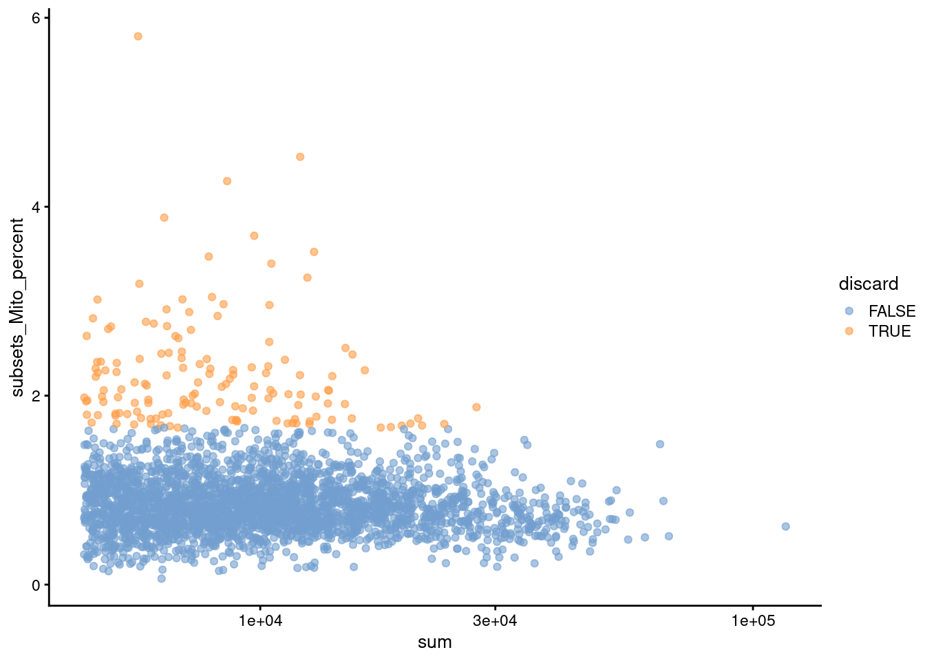
Figure 12.2: Percentage of mitochondrial reads in each cell in the Bach mammary gland dataset compared to its total count. Each point represents a cell and is colored according to whether that cell was discarded.
##              low_lib_size            low_n_features high_subsets_Mito_percent
##                         0                         0                       143
##                   discard
##                       143
12.4 Normalization
library(scran)
set.seed(101000110)
clusters <- quickCluster(sce.mam)
sce.mam <- computeSumFactors(sce.mam, clusters=clusters)
sce.mam <- logNormCounts(sce.mam)## Min. 1st Qu. Median Mean 3rd Qu. Max.
## 0.264 0.520 0.752 1.000 1.207 10.790plot(librarySizeFactors(sce.mam), sizeFactors(sce.mam), pch=16,
xlab="Library size factors", ylab="Deconvolution factors", log="xy")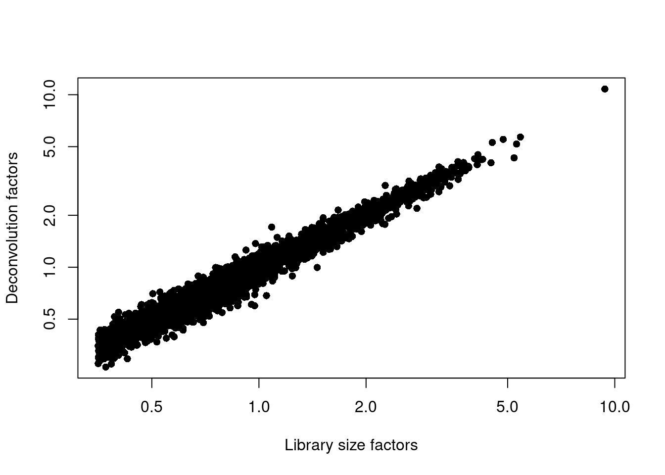
Figure 12.3: Relationship between the library size factors and the deconvolution size factors in the Bach mammary gland dataset.
12.5 Variance modelling
We use a Poisson-based technical trend to capture more genuine biological variation in the biological component.
set.seed(00010101)
dec.mam <- modelGeneVarByPoisson(sce.mam)
top.mam <- getTopHVGs(dec.mam, prop=0.1)plot(dec.mam$mean, dec.mam$total, pch=16, cex=0.5,
xlab="Mean of log-expression", ylab="Variance of log-expression")
curfit <- metadata(dec.mam)
curve(curfit$trend(x), col='dodgerblue', add=TRUE, lwd=2)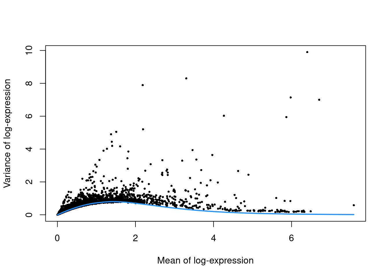
Figure 12.4: Per-gene variance as a function of the mean for the log-expression values in the Bach mammary gland dataset. Each point represents a gene (black) with the mean-variance trend (blue) fitted to simulated Poisson counts.
12.6 Dimensionality reduction
library(BiocSingular)
set.seed(101010011)
sce.mam <- denoisePCA(sce.mam, technical=dec.mam, subset.row=top.mam)
sce.mam <- runTSNE(sce.mam, dimred="PCA")## [1] 1512.7 Clustering
We use a higher k to obtain coarser clusters (for use in doubletCluster() later).
snn.gr <- buildSNNGraph(sce.mam, use.dimred="PCA", k=25)
colLabels(sce.mam) <- factor(igraph::cluster_walktrap(snn.gr)$membership)##
## 1 2 3 4 5 6 7 8 9 10
## 550 847 639 477 54 88 39 22 32 24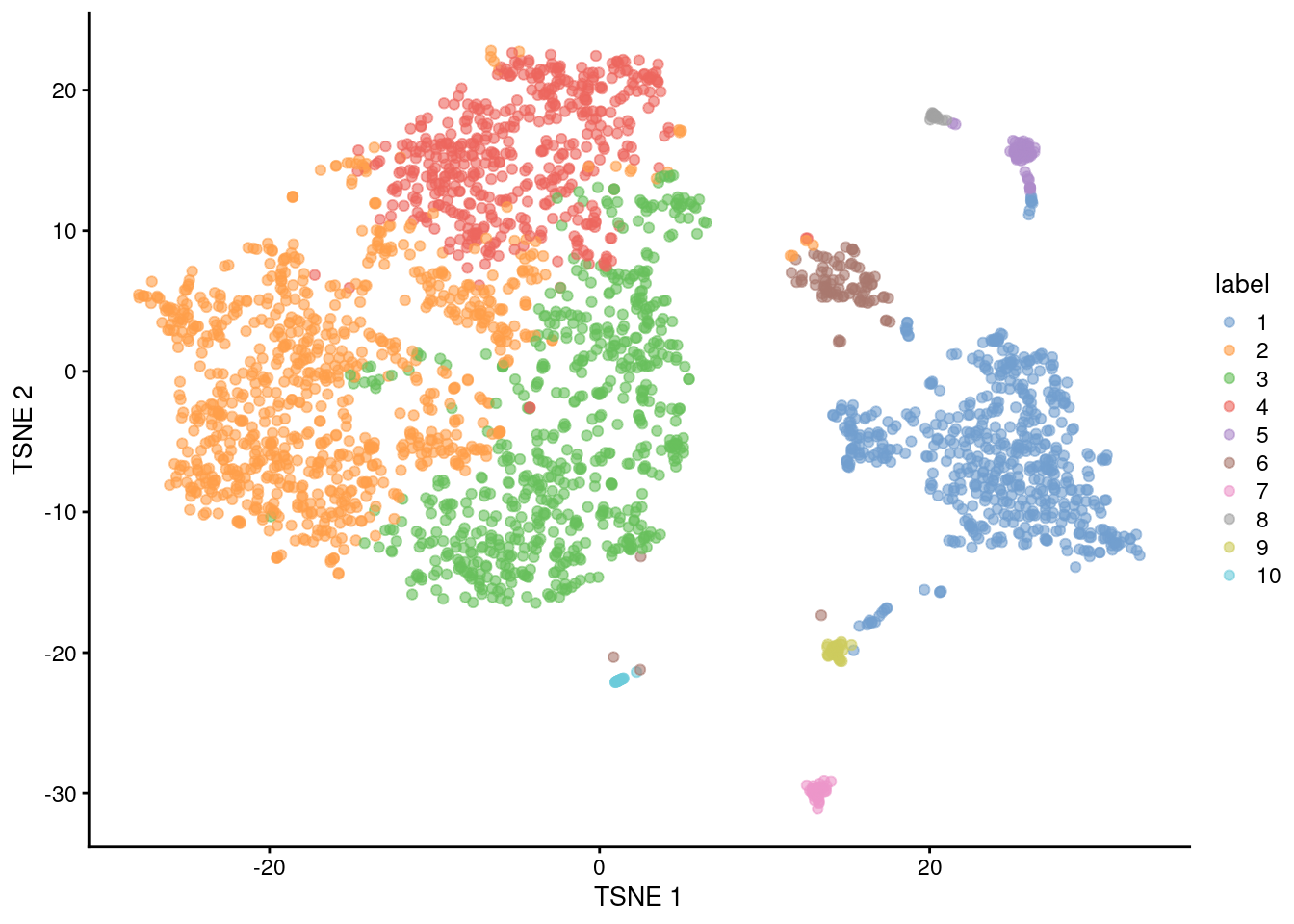
Figure 12.5: Obligatory \(t\)-SNE plot of the Bach mammary gland dataset, where each point represents a cell and is colored according to the assigned cluster.
Session Info
R version 4.4.0 beta (2024-04-15 r86425)
Platform: x86_64-pc-linux-gnu
Running under: Ubuntu 22.04.4 LTS

Matrix products: default
BLAS:   /home/biocbuild/bbs-3.19-bioc/R/lib/libRblas.so
LAPACK: /usr/lib/x86_64-linux-gnu/lapack/liblapack.so.3.10.0

locale:
 [1] LC_CTYPE=en_US.UTF-8       LC_NUMERIC=C
 [3] LC_TIME=en_GB              LC_COLLATE=C
 [5] LC_MONETARY=en_US.UTF-8    LC_MESSAGES=en_US.UTF-8
 [7] LC_PAPER=en_US.UTF-8       LC_NAME=C
 [9] LC_ADDRESS=C               LC_TELEPHONE=C
[11] LC_MEASUREMENT=en_US.UTF-8 LC_IDENTIFICATION=C

time zone: America/New_York
tzcode source: system (glibc)

attached base packages:
[1] stats4    stats     graphics  grDevices utils     datasets  methods
[8] base

other attached packages:
 [1] BiocSingular_1.20.0         scran_1.32.0
 [3] AnnotationHub_3.12.0        BiocFileCache_2.12.0
 [5] dbplyr_2.5.0                scater_1.32.0
 [7] ggplot2_3.5.1               scuttle_1.14.0
 [9] ensembldb_2.28.0            AnnotationFilter_1.28.0
[11] GenomicFeatures_1.56.0      AnnotationDbi_1.66.0
[13] scRNAseq_2.18.0             SingleCellExperiment_1.26.0
[15] SummarizedExperiment_1.34.0 Biobase_2.64.0
[17] GenomicRanges_1.56.0        GenomeInfoDb_1.40.0
[19] IRanges_2.38.0              S4Vectors_0.42.0
[21] BiocGenerics_0.50.0         MatrixGenerics_1.16.0
[23] matrixStats_1.3.0           BiocStyle_2.32.0
[25] rebook_1.14.0

loaded via a namespace (and not attached):
  [1] jsonlite_1.8.8            CodeDepends_0.6.6
  [3] magrittr_2.0.3            ggbeeswarm_0.7.2
  [5] gypsum_1.0.0              farver_2.1.1
  [7] rmarkdown_2.26            BiocIO_1.14.0
  [9] zlibbioc_1.50.0           vctrs_0.6.5
 [11] memoise_2.0.1             Rsamtools_2.20.0
 [13] DelayedMatrixStats_1.26.0 RCurl_1.98-1.14
 [15] htmltools_0.5.8.1         S4Arrays_1.4.0
 [17] curl_5.2.1                BiocNeighbors_1.22.0
 [19] Rhdf5lib_1.26.0           SparseArray_1.4.0
 [21] rhdf5_2.48.0              sass_0.4.9
 [23] alabaster.base_1.4.0      bslib_0.7.0
 [25] alabaster.sce_1.4.0       httr2_1.0.1
 [27] cachem_1.0.8              GenomicAlignments_1.40.0
 [29] igraph_2.0.3              mime_0.12
 [31] lifecycle_1.0.4           pkgconfig_2.0.3
 [33] rsvd_1.0.5                Matrix_1.7-0
 [35] R6_2.5.1                  fastmap_1.1.1
 [37] GenomeInfoDbData_1.2.12   digest_0.6.35
 [39] colorspace_2.1-0          paws.storage_0.5.0
 [41] dqrng_0.3.2               irlba_2.3.5.1
 [43] ExperimentHub_2.12.0      RSQLite_2.3.6
 [45] beachmat_2.20.0           labeling_0.4.3
 [47] filelock_1.0.3            fansi_1.0.6
 [49] httr_1.4.7                abind_1.4-5
 [51] compiler_4.4.0            bit64_4.0.5
 [53] withr_3.0.0               BiocParallel_1.38.0
 [55] viridis_0.6.5             DBI_1.2.2
 [57] highr_0.10                HDF5Array_1.32.0
 [59] alabaster.ranges_1.4.0    alabaster.schemas_1.4.0
 [61] rappdirs_0.3.3            DelayedArray_0.30.0
 [63] bluster_1.14.0            rjson_0.2.21
 [65] tools_4.4.0               vipor_0.4.7
 [67] beeswarm_0.4.0            glue_1.7.0
 [69] restfulr_0.0.15           rhdf5filters_1.16.0
 [71] grid_4.4.0                Rtsne_0.17
 [73] cluster_2.1.6             generics_0.1.3
 [75] gtable_0.3.5              metapod_1.12.0
 [77] ScaledMatrix_1.12.0       utf8_1.2.4
 [79] XVector_0.44.0            ggrepel_0.9.5
 [81] BiocVersion_3.19.1        pillar_1.9.0
 [83] limma_3.60.0              dplyr_1.1.4
 [85] lattice_0.22-6            rtracklayer_1.64.0
 [87] bit_4.0.5                 tidyselect_1.2.1
 [89] paws.common_0.7.2         locfit_1.5-9.9
 [91] Biostrings_2.72.0         knitr_1.46
 [93] gridExtra_2.3             bookdown_0.39
 [95] ProtGenerics_1.36.0       edgeR_4.2.0
 [97] xfun_0.43                 statmod_1.5.0
 [99] UCSC.utils_1.0.0          lazyeval_0.2.2
[101] yaml_2.3.8                evaluate_0.23
[103] codetools_0.2-20          tibble_3.2.1
[105] alabaster.matrix_1.4.0    BiocManager_1.30.22
[107] graph_1.82.0              cli_3.6.2
[109] munsell_0.5.1             jquerylib_0.1.4
[111] Rcpp_1.0.12               dir.expiry_1.12.0
[113] png_0.1-8                 XML_3.99-0.16.1
[115] parallel_4.4.0            blob_1.2.4
[117] sparseMatrixStats_1.16.0  bitops_1.0-7
[119] viridisLite_0.4.2         alabaster.se_1.4.0
[121] scales_1.3.0              purrr_1.0.2
[123] crayon_1.5.2              rlang_1.1.3
[125] cowplot_1.1.3             KEGGREST_1.44.0
References
Bach, K., S. Pensa, M. Grzelak, J. Hadfield, D. J. Adams, J. C. Marioni, and W. T. Khaled. 2017. “Differentiation dynamics of mammary epithelial cells revealed by single-cell RNA sequencing.” Nat Commun 8 (1): 2128.