Chapter 6 Muraro human pancreas (CEL-seq)
6.1 Introduction
This performs an analysis of the Muraro et al. (2016) CEL-seq dataset, consisting of human pancreas cells from various donors.
6.2 Data loading
Converting back to Ensembl identifiers.
library(AnnotationHub)
edb <- AnnotationHub()[["AH73881"]]
gene.symb <- sub("__chr.*$", "", rownames(sce.muraro))
gene.ids <- mapIds(edb, keys=gene.symb,
    keytype="SYMBOL", column="GENEID")

# Removing duplicated genes or genes without Ensembl IDs.
keep <- !is.na(gene.ids) & !duplicated(gene.ids)
sce.muraro <- sce.muraro[keep,]
rownames(sce.muraro) <- gene.ids[keep]
6.3 Quality control
This dataset lacks mitochondrial genes so we will do without. For the one batch that seems to have a high proportion of low-quality cells, we compute an appropriate filter threshold using a shared median and MAD from the other batches (Figure 6.1).
library(scater)
stats <- perCellQCMetrics(sce.muraro)
qc <- quickPerCellQC(stats, percent_subsets="altexps_ERCC_percent",
    batch=sce.muraro$donor, subset=sce.muraro$donor!="D28")
sce.muraro <- sce.muraro[,!qc$discard]colData(unfiltered) <- cbind(colData(unfiltered), stats)
unfiltered$discard <- qc$discard
gridExtra::grid.arrange(
plotColData(unfiltered, x="donor", y="sum", colour_by="discard") +
scale_y_log10() + ggtitle("Total count"),
plotColData(unfiltered, x="donor", y="detected", colour_by="discard") +
scale_y_log10() + ggtitle("Detected features"),
plotColData(unfiltered, x="donor", y="altexps_ERCC_percent",
colour_by="discard") + ggtitle("ERCC percent"),
ncol=2
)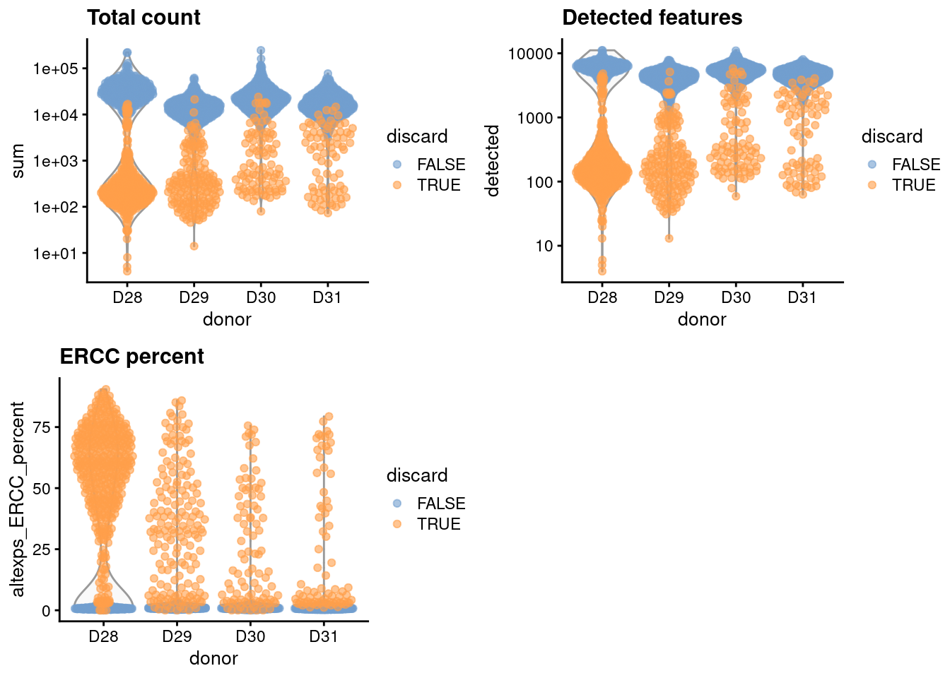
Figure 6.1: Distribution of each QC metric across cells from each donor in the Muraro pancreas dataset. Each point represents a cell and is colored according to whether that cell was discarded.
We have a look at the causes of removal:
##              low_lib_size            low_n_features high_altexps_ERCC_percent
##                       663                       700                       738
##                   discard
##                       773
6.4 Normalization
library(scran)
set.seed(1000)
clusters <- quickCluster(sce.muraro)
sce.muraro <- computeSumFactors(sce.muraro, clusters=clusters)
sce.muraro <- logNormCounts(sce.muraro)## Min. 1st Qu. Median Mean 3rd Qu. Max.
## 0.088 0.541 0.821 1.000 1.211 13.987plot(librarySizeFactors(sce.muraro), sizeFactors(sce.muraro), pch=16,
xlab="Library size factors", ylab="Deconvolution factors", log="xy")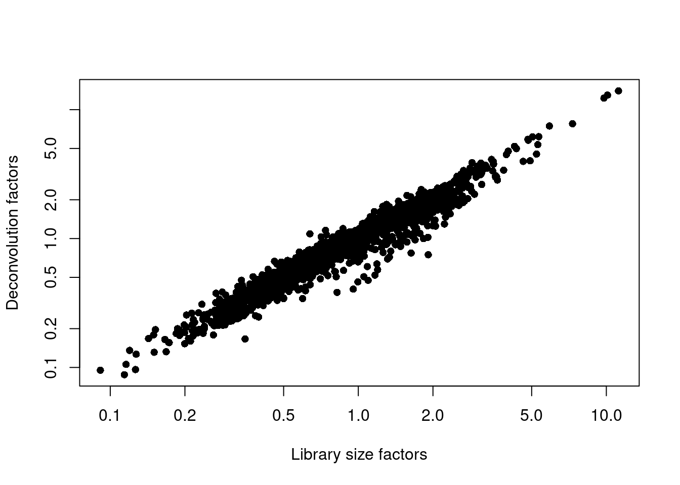
Figure 6.2: Relationship between the library size factors and the deconvolution size factors in the Muraro pancreas dataset.
6.5 Variance modelling
We block on a combined plate and donor factor.
block <- paste0(sce.muraro$plate, "_", sce.muraro$donor)
dec.muraro <- modelGeneVarWithSpikes(sce.muraro, "ERCC", block=block)
top.muraro <- getTopHVGs(dec.muraro, prop=0.1)par(mfrow=c(8,4))
blocked.stats <- dec.muraro$per.block
for (i in colnames(blocked.stats)) {
current <- blocked.stats[[i]]
plot(current$mean, current$total, main=i, pch=16, cex=0.5,
xlab="Mean of log-expression", ylab="Variance of log-expression")
curfit <- metadata(current)
points(curfit$mean, curfit$var, col="red", pch=16)
curve(curfit$trend(x), col='dodgerblue', add=TRUE, lwd=2)
}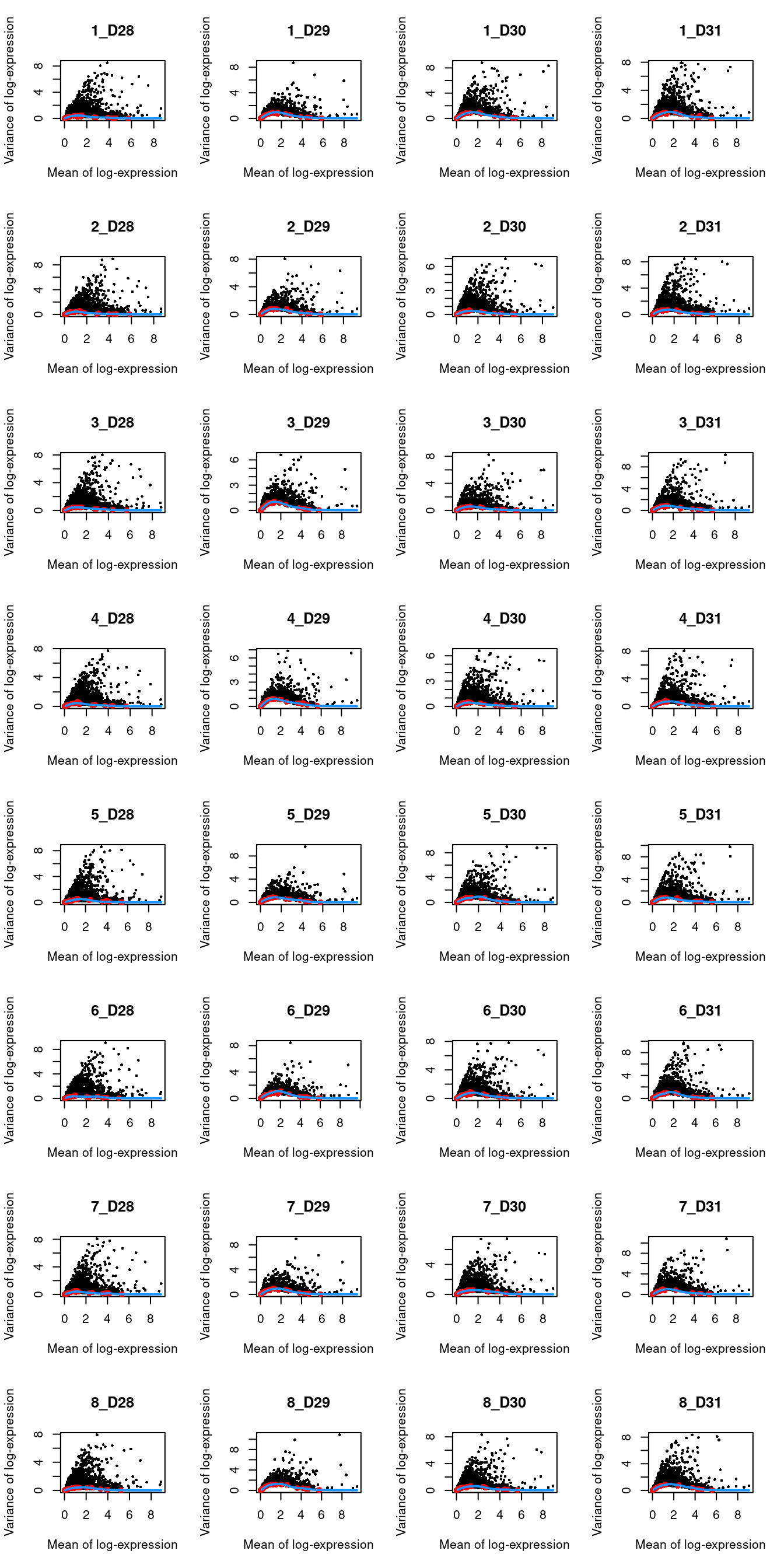
Figure 6.3: Per-gene variance as a function of the mean for the log-expression values in the Muraro pancreas dataset. Each point represents a gene (black) with the mean-variance trend (blue) fitted to the spike-in transcripts (red) separately for each donor.
6.6 Data integration
library(batchelor)
set.seed(1001010)
merged.muraro <- fastMNN(sce.muraro, subset.row=top.muraro,
    batch=sce.muraro$donor)
We use the proportion of variance lost as a diagnostic measure:
##           D28      D29      D30     D31
## [1,] 0.060847 0.024121 0.000000 0.00000
## [2,] 0.002646 0.003018 0.062421 0.00000
## [3,] 0.003449 0.002641 0.002598 0.081626.8 Clustering
snn.gr <- buildSNNGraph(merged.muraro, use.dimred="corrected")
colLabels(merged.muraro) <- factor(igraph::cluster_walktrap(snn.gr)$membership)
tab <- table(Cluster=colLabels(merged.muraro), CellType=sce.muraro$label)
library(pheatmap)
pheatmap(log10(tab+10), color=viridis::viridis(100))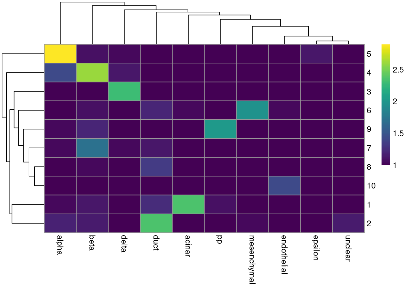
Figure 6.4: Heatmap of the frequency of cells from each cell type label in each cluster.
##        Donor
## Cluster D28 D29 D30 D31
##      1  104   6  57 112
##      2   59  21  77  97
##      3   12  75  64  43
##      4   28 149 126 120
##      5   87 261 277 214
##      6   21   7  54  26
##      7    1   6   6  37
##      8    6   6   5   2
##      9   11  68   5  30
## 10 4 2 5 8gridExtra::grid.arrange(
plotTSNE(merged.muraro, colour_by="label"),
plotTSNE(merged.muraro, colour_by="batch"),
ncol=2
)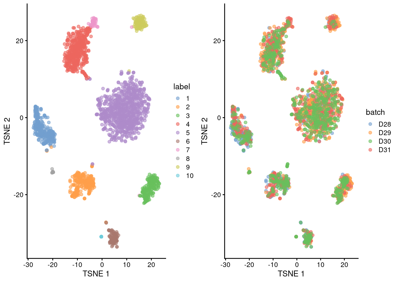
Figure 6.5: Obligatory \(t\)-SNE plots of the Muraro pancreas dataset. Each point represents a cell that is colored by cluster (left) or batch (right).
Session Info
R version 4.3.0 RC (2023-04-13 r84269)
Platform: x86_64-pc-linux-gnu (64-bit)
Running under: Ubuntu 22.04.2 LTS

Matrix products: default
BLAS:   /home/biocbuild/bbs-3.17-bioc/R/lib/libRblas.so
LAPACK: /usr/lib/x86_64-linux-gnu/lapack/liblapack.so.3.10.0

locale:
 [1] LC_CTYPE=en_US.UTF-8       LC_NUMERIC=C
 [3] LC_TIME=en_GB              LC_COLLATE=C
 [5] LC_MONETARY=en_US.UTF-8    LC_MESSAGES=en_US.UTF-8
 [7] LC_PAPER=en_US.UTF-8       LC_NAME=C
 [9] LC_ADDRESS=C               LC_TELEPHONE=C
[11] LC_MEASUREMENT=en_US.UTF-8 LC_IDENTIFICATION=C

time zone: America/New_York
tzcode source: system (glibc)

attached base packages:
[1] stats4    stats     graphics  grDevices utils     datasets  methods
[8] base

other attached packages:
 [1] pheatmap_1.0.12             batchelor_1.16.0
 [3] scran_1.28.0                scater_1.28.0
 [5] ggplot2_3.4.2               scuttle_1.10.0
 [7] ensembldb_2.24.0            AnnotationFilter_1.24.0
 [9] GenomicFeatures_1.52.0      AnnotationDbi_1.62.0
[11] AnnotationHub_3.8.0         BiocFileCache_2.8.0
[13] dbplyr_2.3.2                scRNAseq_2.13.0
[15] SingleCellExperiment_1.22.0 SummarizedExperiment_1.30.0
[17] Biobase_2.60.0              GenomicRanges_1.52.0
[19] GenomeInfoDb_1.36.0         IRanges_2.34.0
[21] S4Vectors_0.38.0            BiocGenerics_0.46.0
[23] MatrixGenerics_1.12.0       matrixStats_0.63.0
[25] BiocStyle_2.28.0            rebook_1.10.0

loaded via a namespace (and not attached):
  [1] RColorBrewer_1.1-3            jsonlite_1.8.4
  [3] CodeDepends_0.6.5             magrittr_2.0.3
  [5] ggbeeswarm_0.7.1              farver_2.1.1
  [7] rmarkdown_2.21                BiocIO_1.10.0
  [9] zlibbioc_1.46.0               vctrs_0.6.2
 [11] memoise_2.0.1                 Rsamtools_2.16.0
 [13] DelayedMatrixStats_1.22.0     RCurl_1.98-1.12
 [15] htmltools_0.5.5               progress_1.2.2
 [17] curl_5.0.0                    BiocNeighbors_1.18.0
 [19] sass_0.4.5                    bslib_0.4.2
 [21] cachem_1.0.7                  ResidualMatrix_1.10.0
 [23] GenomicAlignments_1.36.0      igraph_1.4.2
 [25] mime_0.12                     lifecycle_1.0.3
 [27] pkgconfig_2.0.3               rsvd_1.0.5
 [29] Matrix_1.5-4                  R6_2.5.1
 [31] fastmap_1.1.1                 GenomeInfoDbData_1.2.10
 [33] shiny_1.7.4                   digest_0.6.31
 [35] colorspace_2.1-0              dqrng_0.3.0
 [37] irlba_2.3.5.1                 ExperimentHub_2.8.0
 [39] RSQLite_2.3.1                 beachmat_2.16.0
 [41] labeling_0.4.2                filelock_1.0.2
 [43] fansi_1.0.4                   httr_1.4.5
 [45] compiler_4.3.0                bit64_4.0.5
 [47] withr_2.5.0                   BiocParallel_1.34.0
 [49] viridis_0.6.2                 DBI_1.1.3
 [51] highr_0.10                    biomaRt_2.56.0
 [53] rappdirs_0.3.3                DelayedArray_0.26.0
 [55] bluster_1.10.0                rjson_0.2.21
 [57] tools_4.3.0                   vipor_0.4.5
 [59] beeswarm_0.4.0                interactiveDisplayBase_1.38.0
 [61] httpuv_1.6.9                  glue_1.6.2
 [63] restfulr_0.0.15               promises_1.2.0.1
 [65] grid_4.3.0                    Rtsne_0.16
 [67] cluster_2.1.4                 generics_0.1.3
 [69] gtable_0.3.3                  hms_1.1.3
 [71] metapod_1.8.0                 BiocSingular_1.16.0
 [73] ScaledMatrix_1.8.0            xml2_1.3.3
 [75] utf8_1.2.3                    XVector_0.40.0
 [77] ggrepel_0.9.3                 BiocVersion_3.17.1
 [79] pillar_1.9.0                  stringr_1.5.0
 [81] limma_3.56.0                  later_1.3.0
 [83] dplyr_1.1.2                   lattice_0.21-8
 [85] rtracklayer_1.60.0            bit_4.0.5
 [87] tidyselect_1.2.0              locfit_1.5-9.7
 [89] Biostrings_2.68.0             knitr_1.42
 [91] gridExtra_2.3                 bookdown_0.33
 [93] ProtGenerics_1.32.0           edgeR_3.42.0
 [95] xfun_0.39                     statmod_1.5.0
 [97] stringi_1.7.12                lazyeval_0.2.2
 [99] yaml_2.3.7                    evaluate_0.20
[101] codetools_0.2-19              tibble_3.2.1
[103] BiocManager_1.30.20           graph_1.78.0
[105] cli_3.6.1                     xtable_1.8-4
[107] munsell_0.5.0                 jquerylib_0.1.4
[109] Rcpp_1.0.10                   dir.expiry_1.8.0
[111] png_0.1-8                     XML_3.99-0.14
[113] parallel_4.3.0                ellipsis_0.3.2
[115] blob_1.2.4                    prettyunits_1.1.1
[117] sparseMatrixStats_1.12.0      bitops_1.0-7
[119] viridisLite_0.4.1             scales_1.2.1
[121] purrr_1.0.1                   crayon_1.5.2
[123] rlang_1.1.0                   cowplot_1.1.1
[125] KEGGREST_1.40.0
References
Muraro, M. J., G. Dharmadhikari, D. Grun, N. Groen, T. Dielen, E. Jansen, L. van Gurp, et al. 2016. “A Single-Cell Transcriptome Atlas of the Human Pancreas.” Cell Syst 3 (4): 385–94.